Reinforcement Learning-Based Model Matching in COBRA, a Slithering Snake Robot
a byte-sized version of my master's thesis
Abstract
This work employs a reinforcement learning-based model identification method aimed at enhancing the accuracy of the dynamics for our snake robot, called COBRA. Leveraging gradient information and iterative optimization, the proposed approach refines the parameters of COBRA’s dynamical model such as coefficient of friction and actuator parameters using experimental and simulated data. Experimental validation on the hardware platform demonstrates the efficacy of the proposed approach, highlighting its potential to address sim-to-real gap in robot implementation. The full report with proper citations and in-depth analysis is available here.
Introduction
Simulation-to-Reality Gap
Developing effective locomotion controllers for mobile robots is challenging, and while Deep Reinforcement Learning (DRL) offers promising solutions, it requires impractical amounts of training data for high-risk tasks like locomotion and manipulation. Although computer simulations provide a safe and efficient training environment, the resulting policies often fail to transfer effectively to real hardware due to the “Simulation-to-Reality Gap” (sim2real gap), caused by discrepancies such as differences in friction, joint dynamics, and sensor noise between simulated and real environments. These discrepancies impede the transition of control policies from simulation to real-world applications, resulting in suboptimal performance and limited generalization of robotic systems.
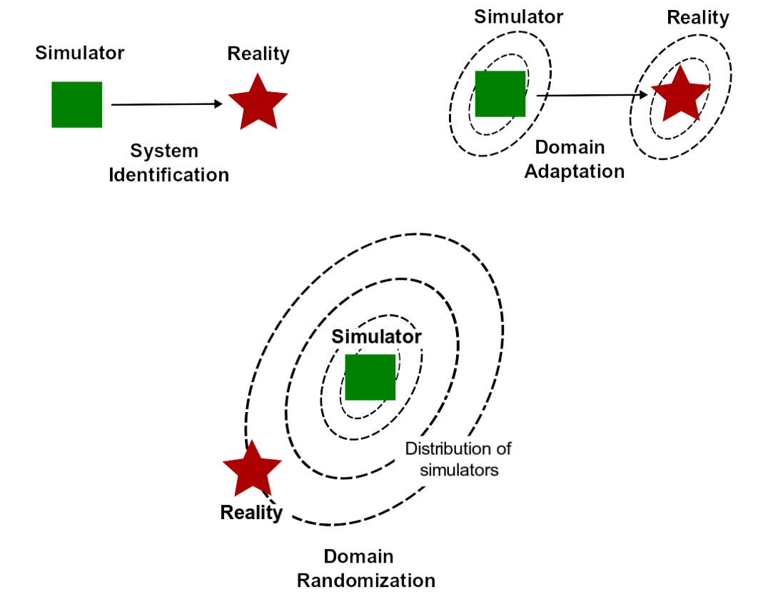
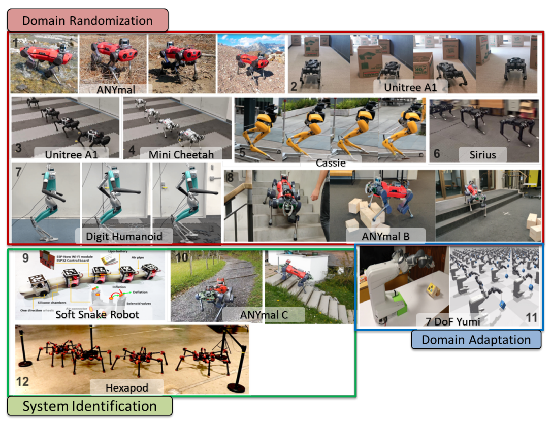
To tackle the challenges of the Simulation-to-Reality Gap, recent research has focused on several advanced strategies. These include employing more sophisticated system identification procedures to improve model accuracy, training policies on real robots while simultaneously enhancing simulator accuracy through domain adaptation, and developing robust control policies that can generalize across varied simulated environments through domain randomization. Although these methods have shown good transferability of learned policies from simulation to real robots, they typically require at least 1000 hours of training in the simulator and/or hundreds of rollouts on the real robot. The figure below highlights several state-of-the-art solutions addressing the sim2real problem across various robots.
Motivation
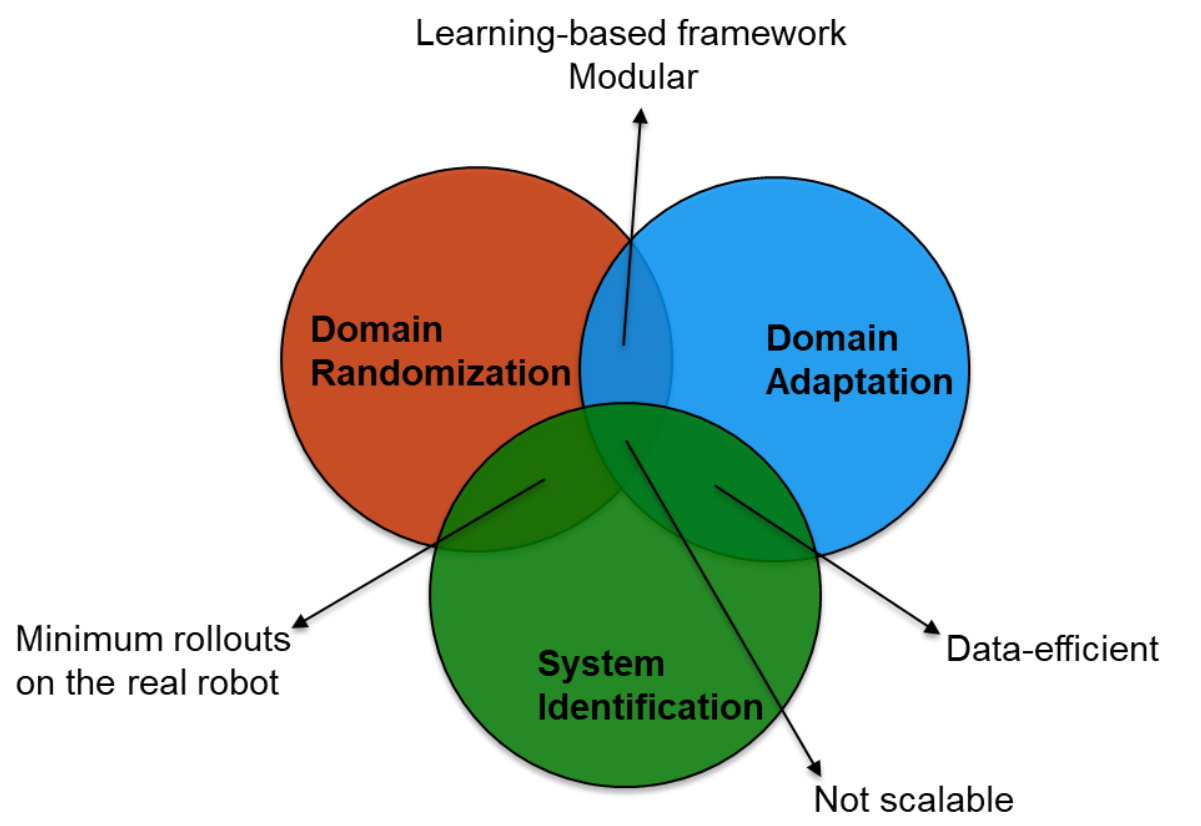
Significant progress has been made in simulation-to-reality transfer for locomotion tasks, but several research gaps remain. There is a strong motivation to develop a framework which:
- is data-efficient
- is learning-based
- is scalable
- is modular
- requires minimum rollouts on the real robot
- has standardized evaluation metrics for sim2real transfer
Simulators and Physics Engines
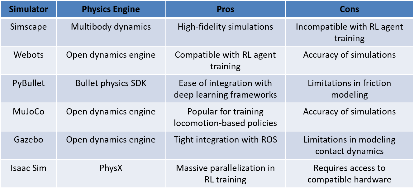
Table 1 compares pros and cons of most widely used physics simulators for robotics applications. After considering all the options, I chose the Webots simulator as the ideal platform for bridging the sim2real gap in training reinforcement learning (RL) agents for the COBRA platform due to its robust integration capabilities with RL training and extensive resources for developing locomotion, manipulation, and navigation controllers. Webots offers a user-friendly interface and supports various programming languages like Python and C++, simplifying the implementation and integration of RL algorithms. Its diverse library of robot models, realistic physics simulations, and advanced visualization tools create an optimal environment for training RL-based locomotion policies.
Additionally, Webots provides comprehensive tools and resources for developing controllers for various tasks essential to the COBRA platform’s functionality. Overall, Webots’ compatibility with RL training and its rich resources make it an excellent choice for addressing the sim2real gap in developing efficient controllers for the COBRA platform.
COBRA Platform

COBRA, short for Crater Observing Bio-inspired Rolling Articulator, is a snake robot inspired by the movement of serpentine creatures. Engineered to navigate rugged terrains like craters, where traditional robots may struggle, COBRA features 11 joints and 12 links, providing complex and versatile movements. Its 6 yawing and 5 pitching joints allow a wide range of orientations, making it suitable for diverse robotic applications. The free body diagram provides a detailed representation of the forces and moments acting on the COBRA platform as it interacts with the ground. The coefficients of friction play a crucial role in analyzing the stability and motion dynamics of the platform during various maneuvers. The ground contact model used in the simulator is given below:
\[F_{GRF} = \begin{cases} 0, & \text{if } p_{C,z} > 0\\ [F_{GRF,x},F_{GRF,y},F_{GRF,z}]^T,& \text{otherwise} \end{cases}\] \[F_{GRF,i} = - s_{i} F_{GRF,z} \, \mathrm{sgn}(\dot p_{C,i}) - \mu_v \dot p_{C,i} ~~ \mbox{if} ~~i=x, y\] \[F_{GRF,z} = -k_1 p_{C,z} - k_{2} \dot p_{C,z}\] \[s_{i} = \Big(\mu_c - (\mu_c - \mu_s) \mathrm{exp} \left(-|\dot p_{C,i}|^2/v_s^2 \right) \Big)\]where \(p_{C,i}\), \(i = x, y, z\), are the \(x - y - z\) positions of the contact point; \(F_{GRF,i}\), \(i = x, y, z\), are the \(x - y - z\) components of the ground reaction force, assuming contact occurs between the robot and the ground substrate. The force terms are given by, \(k_1\) and \(k_2\) are the spring and damping coefficients of the compliant surface model. The term \(s_i\) is defined by \(\mu_c\), \(\mu_s\), and \(\mu_v\), which are the Coulomb, static, and viscous friction coefficients, with \(v_s > 0\) being the Stribeck velocity. Specifically, the unknown parameters include actuator model parameters and Stribeck terms.
Central Pattern Generators
Central Pattern Generators (CPGs) are neural networks in the spinal cord and brainstem of vertebrates, including humans, responsible for generating rhythmic neural activity that coordinates repetitive motor movements like walking, swimming, and breathing, without continuous input from higher brain centers. CPGs are crucial for locomotion and other rhythmic behaviors, producing rhythmic patterns even without sensory feedback or external stimuli. This autonomous rhythmicity allows for automatic and adaptive rhythmic movements without constant conscious control.
In research and robotics, CPGs are studied for their potential in biomimetic control of locomotion and other behaviors in artificial systems. By modeling CPG principles in artificial neural networks, researchers can create control systems that mimic biological rhythmicity, integrating these artificial CPGs into robotic systems for autonomous and efficient control of locomotion, navigation, and other motor functions.
Modified Kuramoto Model
The Kuramoto CPG model is a mathematical framework for describing rhythmic oscillatory behavior in biological systems, particularly for robotic locomotion control, by using coupled phase oscillators to generate synchronized and coordinated rhythmic patterns. I used a modified version of the original Kuramoto model, with the dynamics detailed below.
\[\dot{\varphi} = \omega + A \cdot \varphi + B \cdot \theta\] \[\ddot{r} = a \cdot [\frac{a}{4} \cdot (R - r) - \dot{r}]\] \[x = r \cdot \sin(\varphi) + \delta\] \[A = \begin{bmatrix} -\mu_1 & \mu_1 \\ \mu_2 & -2\mu_2 & \mu_2 \\ & & \ddots & \\ & & \mu_{n-1} & -2\mu_{n-1} & \mu_{n-1} \\ & & & \mu_n & -\mu_n \\ \end{bmatrix}\] \[B = \begin{bmatrix} 1 \\ -1 & 1 \\ & -1 & \ddots \\ & & \ddots & 1 \\ & & & -1 & 1 \\ & & & & -1 \\ \end{bmatrix}\]Where \(\varphi \in \mathbb{R}^n\) and \(r \in \mathbb{R}^n\) are the internal states of the CPG, \(n\) is the number of output channels (usually equal to the number of robot joints), \(a\) and \(\mu_i\) are hyperparameters controlling the convergence rate, \(R \in \mathbb{R}^n\), \(\omega \in \mathbb{R}^n\), \(\theta \in \mathbb{R}^{n-1}\), \(\delta \in \mathbb{R}^n\) are inputs controlling the desired amplitude, frequency, phase shift, and offset, and \(x \in \mathbb{R}^n\) is the output sinusoidal waves of \(n\) channels.
Model Matching Framework
Sidewinding Experiment
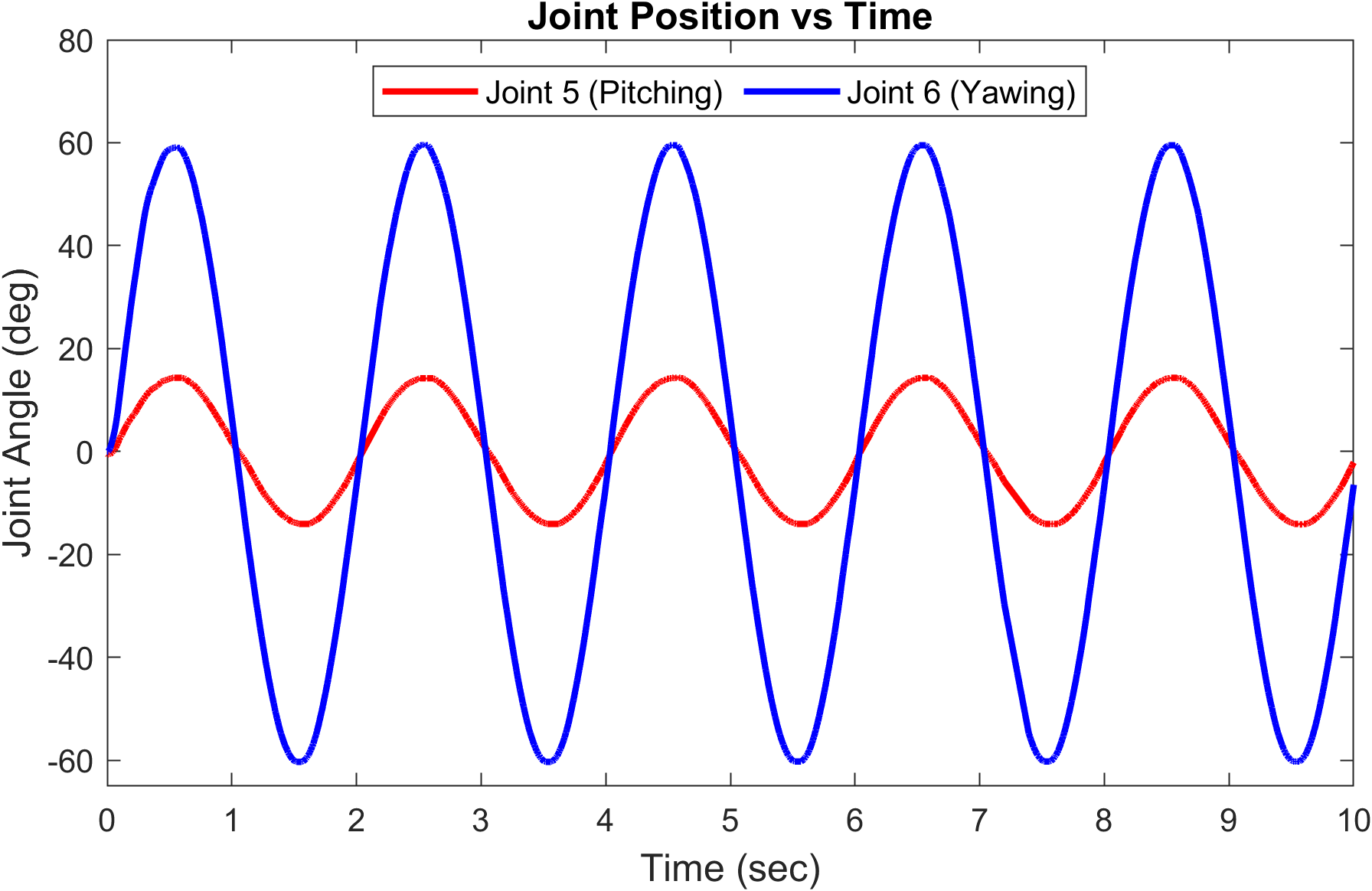
The left clip of Video 2 illustrates the COBRA platform sidewinding on flat ground. The sidewinding trajectory is generated by the sine equation:
\[y(t) = A \sin(\omega t + \phi)\]where \(y(t)\) represents the lateral position of the COBRA platform at time \(t, A\) is the amplitude of the sidewinding motion, \(\omega\) is the angular frequency, and \(\phi\) is the phase angle. Figure 6 shows the data collected from the real robot.
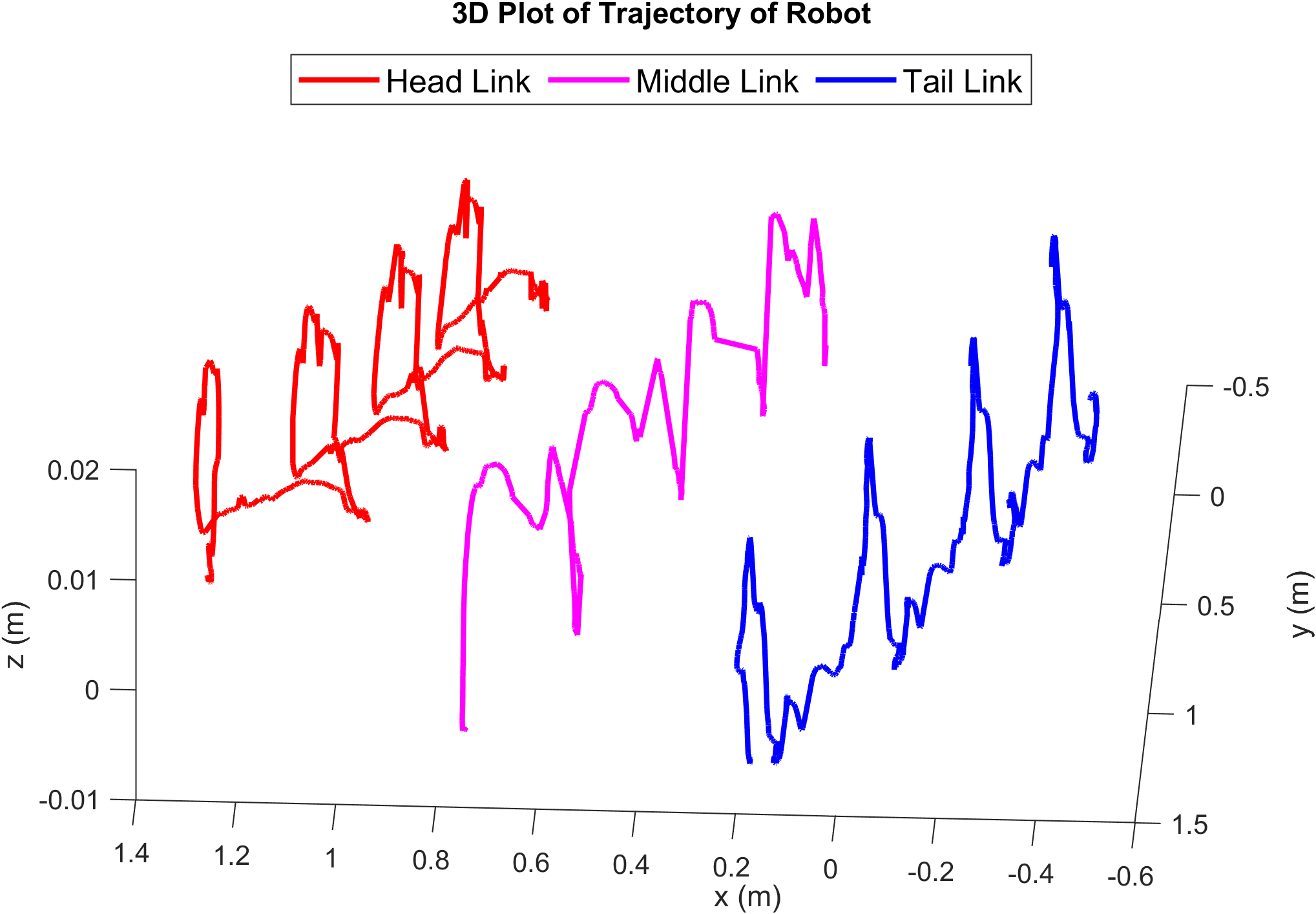

The simulation-to-reality gap observed in the Webots simulator is highlighted in experiments conducted on the physical robot (Video 2). Motion capture technology recorded the trajectories of the head, tail, and middle links, along with joint trajectory data for all eleven joints. Odd-numbered joints executed pitching motions, while even-numbered joints executed yawing motions. A sidewinding gait was generated using a sinusoidal input signal to each joint, with adjustable parameters to modify the robot’s behavior. The input signal followed a sine-wave pattern with varying phase differences applied to each joint:
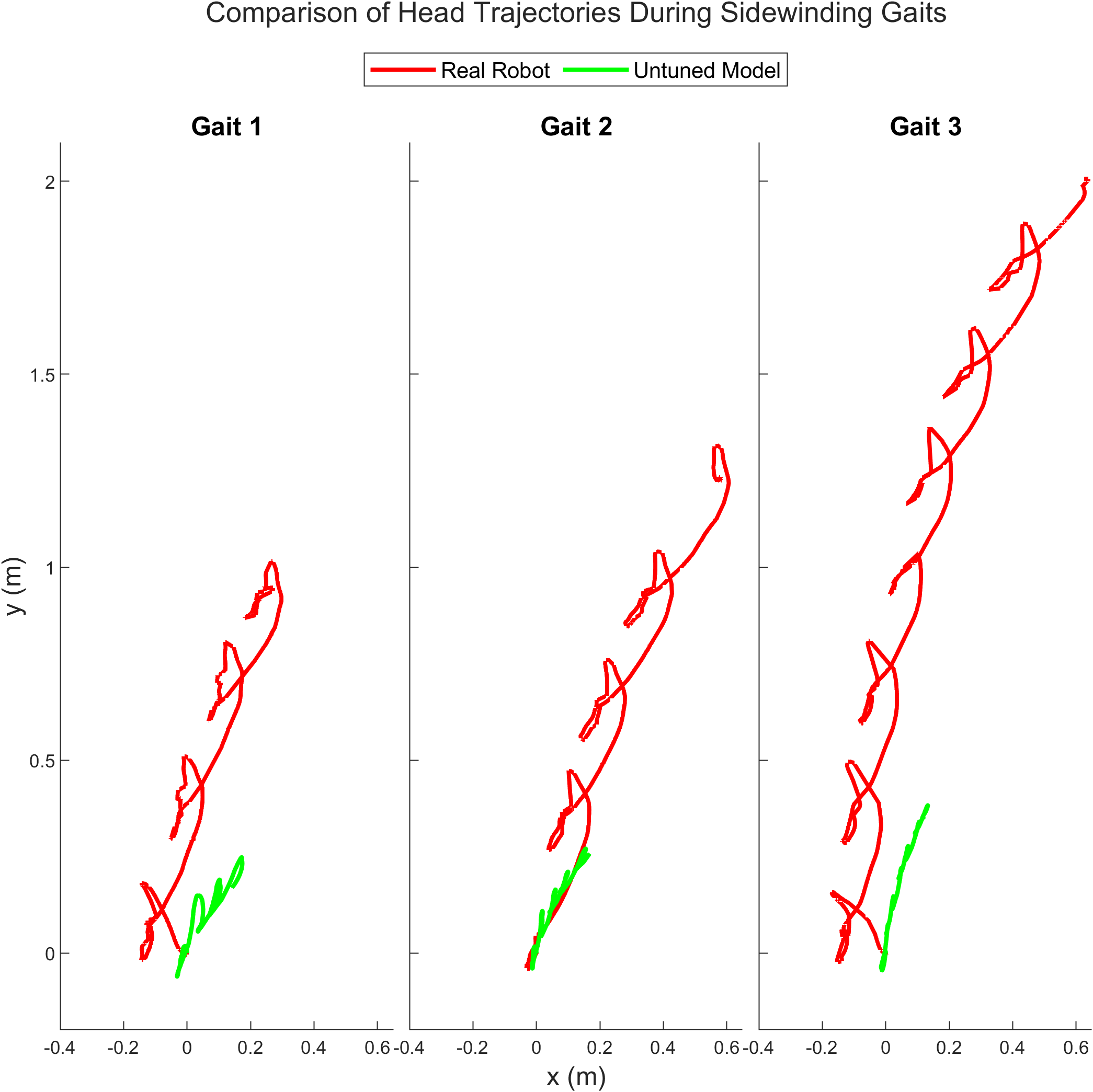
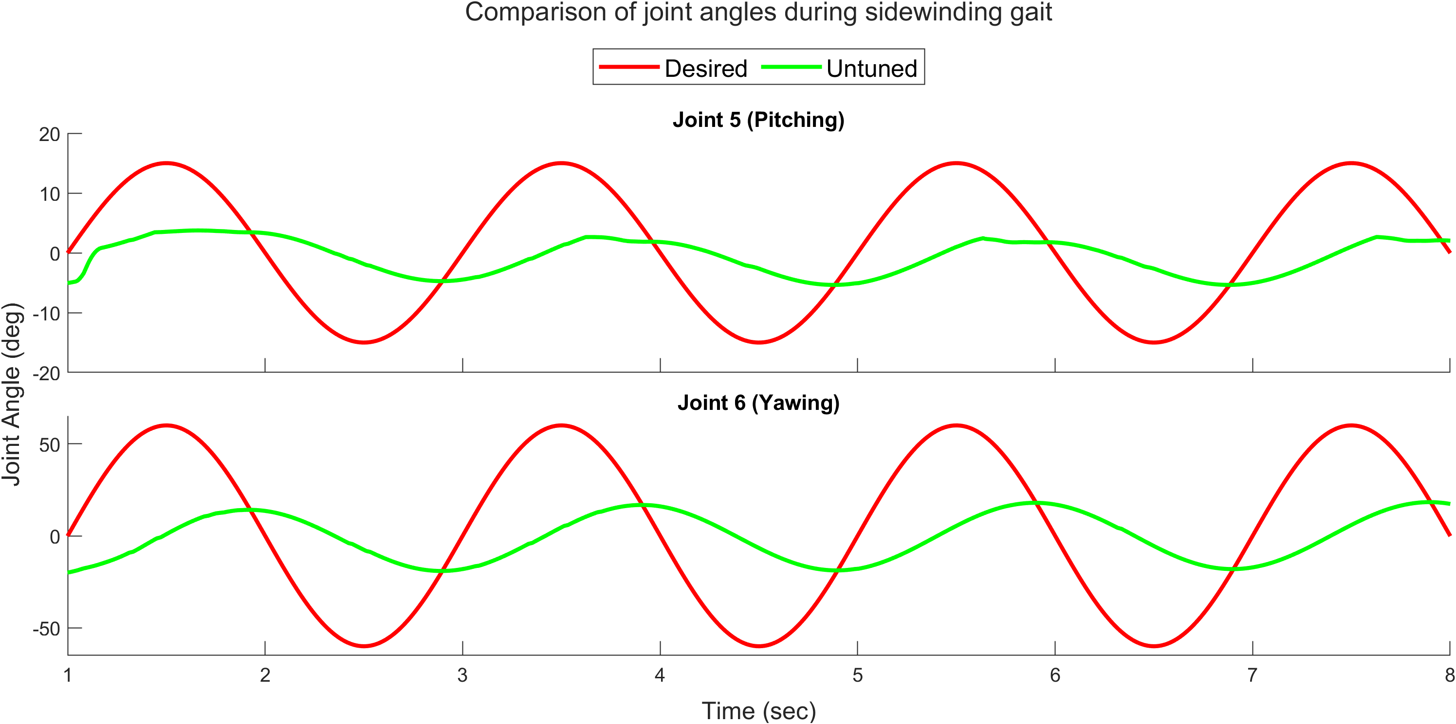
\[A_{pitching} = 14^\circ, A_{yawing} = 60^\circ\] \[\phi = \frac{\pi}{2} [0, 0, 1, 1, 2, 2, 3, 3, 0, 0, 1]\]The identical trajectory was also executed in the Webots simulator, allowing observation of the discrepancy between the simulator and the actual robot. This disparity is more evident in Figure 7, which compares the head trajectories over time for three different gait patterns in both the actual robot and the base simulator (untuned model). Gait 1 represents sidewinding at 0.35 Hz, Gait 2 at 0.5 Hz, and Gait 3 at 0.65 Hz. Additionally, Figure 8 highlights how the performance of the actuator model also contributes to the gap between simulation and reality. These disparities hinder the seamless transfer of control policies from simulation to the real robot, limiting the effectiveness of learned behaviors in practical applications. Addressing the sim-to-real issue is crucial for ensuring COBRA’s reliability and robustness in diverse and dynamic environments.
Methodology
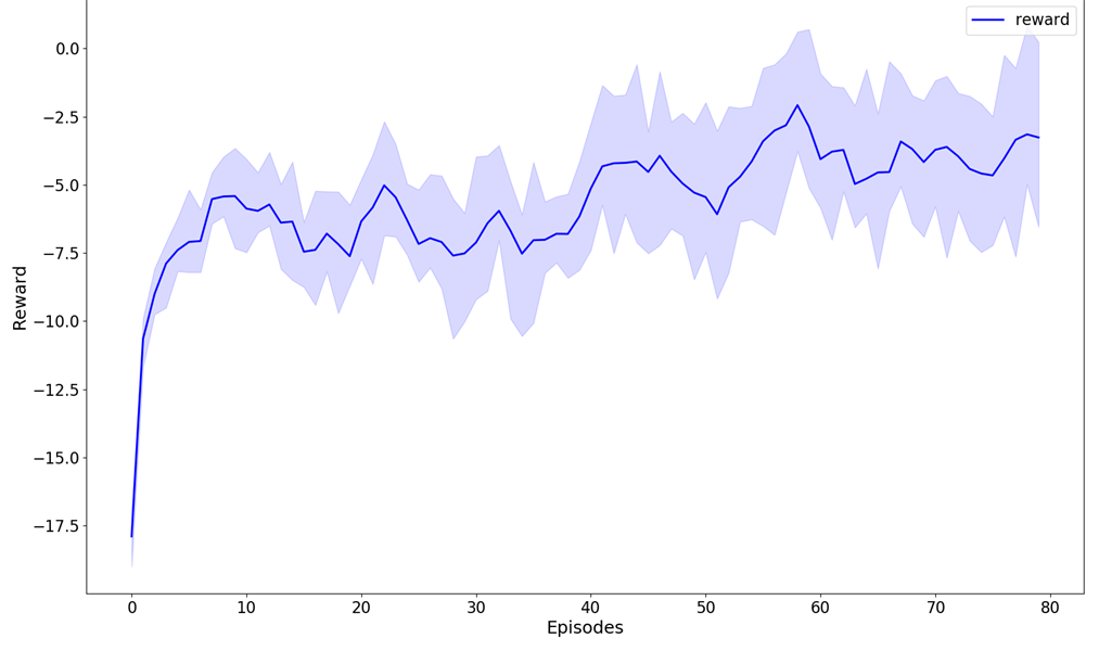
The proposed model matching framework (Fig. 9) is designed to tune the dynamic model and identify accurate parameters that minimize the disparity between simulation and reality using a reinforcement learning-based method. Our methodology involved executing a predetermined sidewinding trajectory (operating at 0.5 Hz) on both the physical COBRA robot and the Webots simulator. A sidewinding trajectory command guided both systems through identical movements. Performance analysis was conducted in two domains: underactuated dynamics, which involved comparing the head’s position and orientation to identify contact force discrepancies, and actuated dynamics, focusing on joint angle trajectories to evaluate movement precision. Positional data for the head, middle link, tail, and joints were collected during the sidewinding gait. Alignment between simulation and reality was quantified using a reward function, and a reinforcement learning agent adjusted model parameters to maximize this function, aiming to minimize the sim2real gap. Proximal Policy Optimization (PPO) algorithm is used to iteratively refine the simulation model.
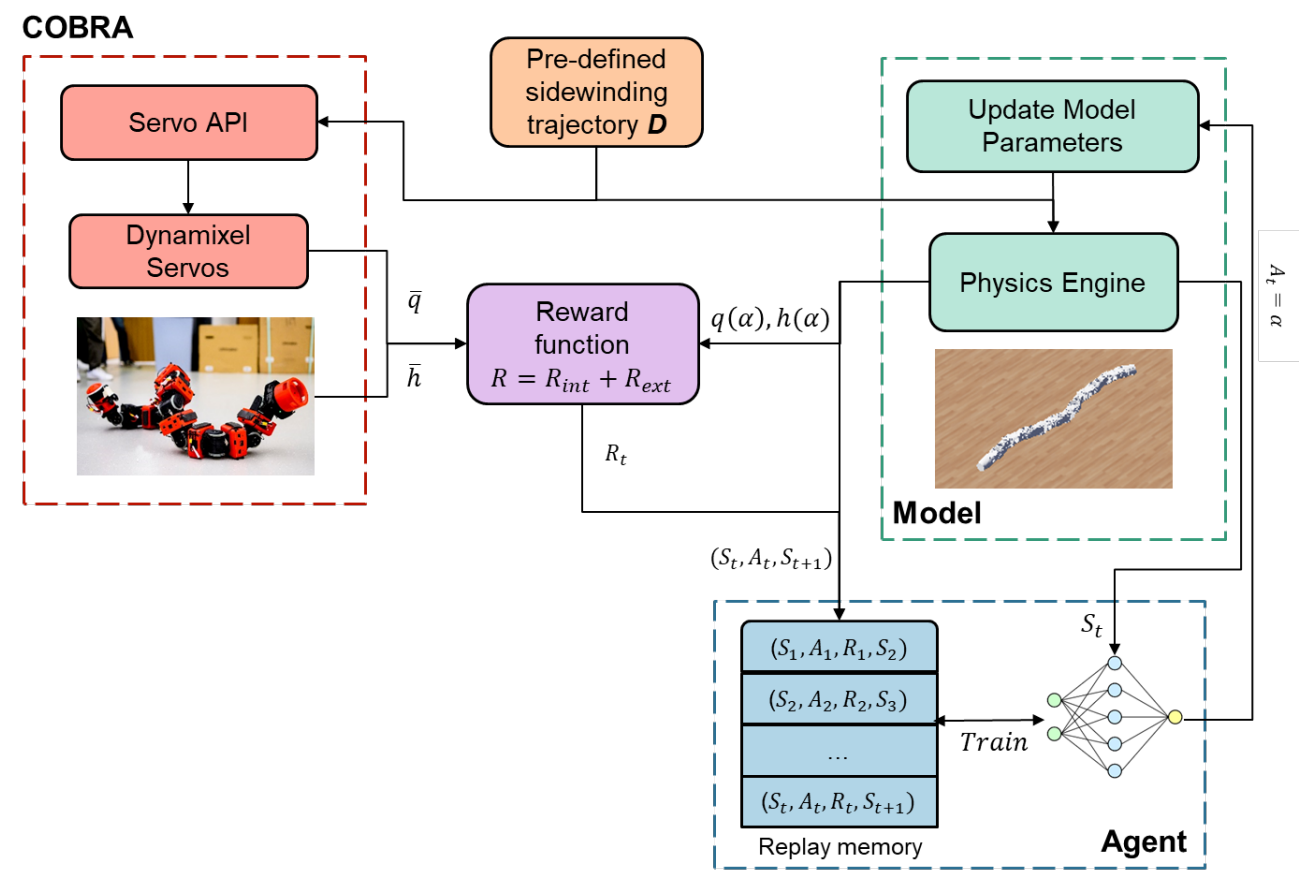
The state \(S_t\) includes actuator parameters for internal tuning and Stribeck terms for external tuning. The actions \(A_t\) are adjustments to these simulation parameters.
\[S = [h(\alpha), \bar{h}, q(\alpha), \bar{q}, \mu, K_p, K_i, K_d]\]where \(h(\alpha), \bar{h}, q(\alpha), \bar{q}\) represent head trajectory from simulation, head trajectory from real robot, joint trajectories from simulation and joint trajectories from real robot. \(K_p, K_i, K_d\) represent PID gain values of the actuator model of the robot in simulator.
The reward function \(R = R_{\text{int}} + R_{\text{ext}}\) is defined as:
\[R_{\text{external}} = - \sqrt{(x_{\text{des}} - x_{\text{actual}})^2 + (y_{\text{des}} - y_{\text{actual}})^2}\]where \(x_{\text{des}}\) and \(y_{\text{des}}\) are the desired x- and y-positions of the head module, and \(x_{\text{actual}}\) and \(y_{\text{actual}}\) are the actual positions from OptiTrack data.
The internal reward \(R_{\text{internal}}\) is given by:
\[R_{\text{internal}} = - (\phi_{\text{des}} - \phi_{\text{actual}})^2 - (\omega_{\text{des}} - \omega_{\text{actual}})^2 - (A_{\text{des}} - A_{\text{actual}})^2\]where \(\phi\), \(\omega\), and \(A\) are CPG variables. These reward functions are designed to penalize deviations in both passive and actuated dynamics, using the L$^2$-norm of the differences in joint angle trajectories and the final head position.
During the training phase, the policy network is updated with new data, with PPO adjusting the policy to maximize cumulative rewards while preserving similarity to the previous policy. This is achieved through a mechanism known as clipping, which prevents drastic policy changes. The results of the tuning procedure are presented in the results section.
Loco-manipulation Controller
Motivation
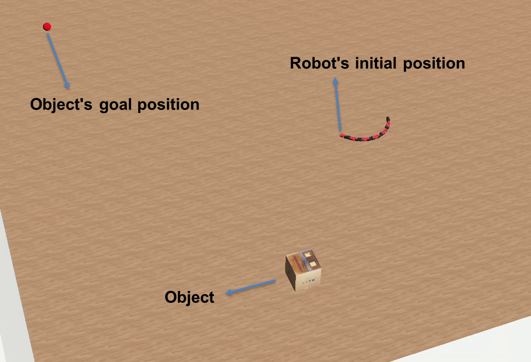
The tuned model derived from the Model Matching framework provides valuable capabilities for developing advanced locomotion strategies that can be transferred to the real robot. One such strategy is Loco-manipulation, which involves manipulating objects in the robot’s vicinity during locomotion tasks. This technique is especially significant for the COBRA platform, leveraging its unique design to enhance dexterity and precision in object manipulation. By integrating locomotion and manipulation seamlessly, COBRA can increase its functionality and adaptability across various tasks, boosting overall efficiency and versatility. In the following sections, I introduce the Loco-manipulation controller, detailing its design and functionality. Although this controller addresses the specified problem effectively, it is important to note that the current version cannot be directly transferred to the real robot because the locomotion policy was trained using an untuned model.
Methodology
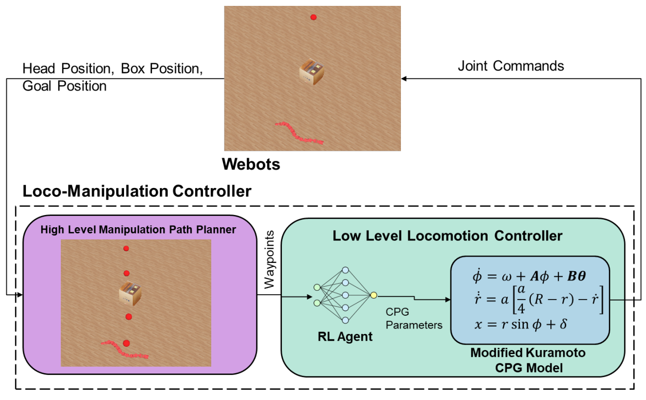
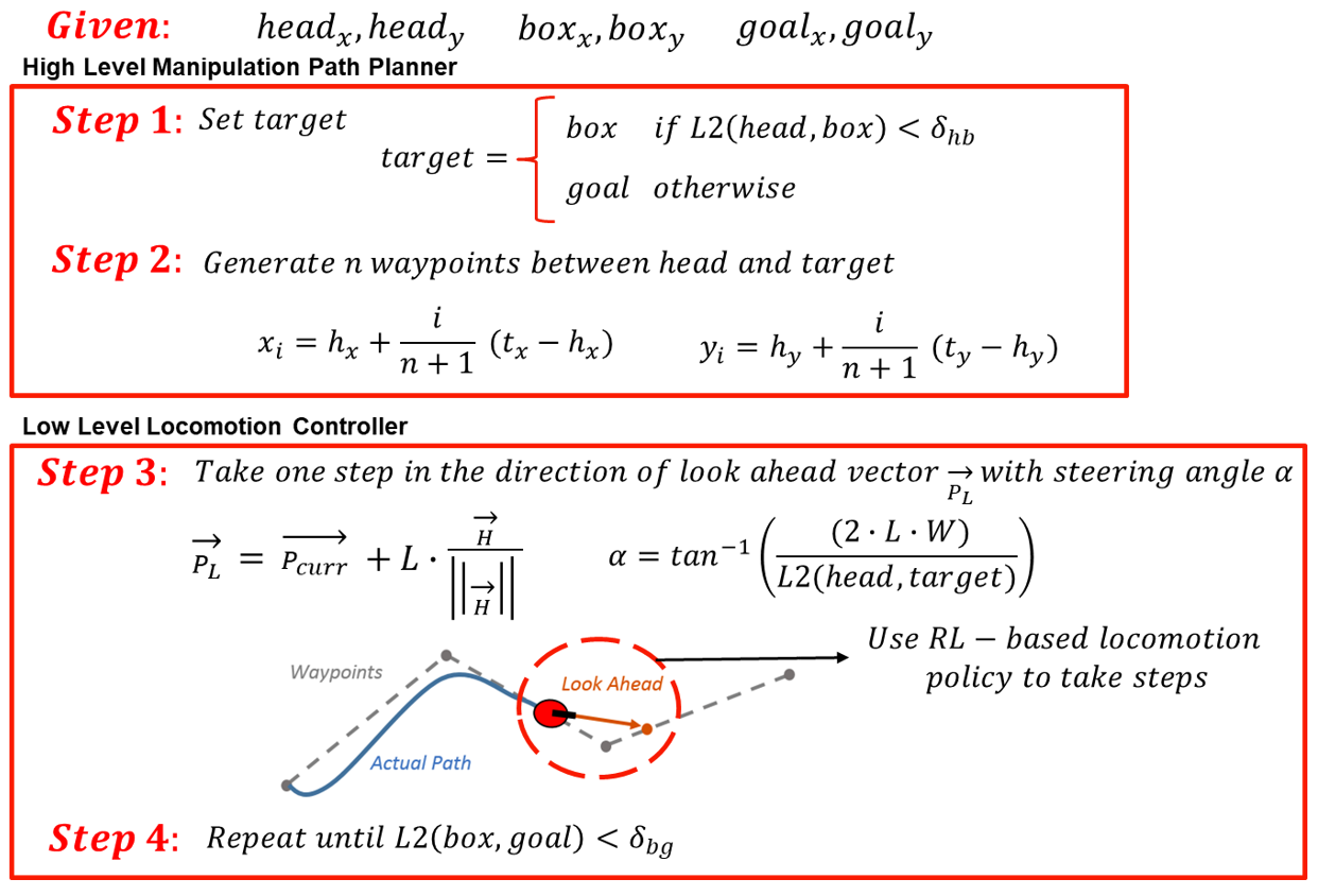
The hierarchical framework for developing the loco-manipulation controller is illustrated in Fig. 11. This structure simplifies the problem by dividing it into two parts, detailed step-by-step in Algorithm 1. The high-level manipulation path planner (steps 1 and 2 in the algorithm) plans the trajectory from the robot’s head position to designated goal positions, ensuring the robot can effectively manipulate an object from its initial location to the target. This planner creates waypoints along the path and sends them to the low-level locomotion controller (steps 3 and 4 in algorithm). The low-level locomotion controller receives these waypoints and executes them using a locomotion policy trained with reinforcement learning. This policy generates parameters for the modified kuramoto CPG model, which determines the joint positions necessary for the robot’s movements. Results and analysis of the loco-manipulation controller are presented in results section.
Results
Model Matching
Video 4 shows the robot performing a sidewinding gait at 0.5 Hz, highlighting the impact of model tuning, with the red dot indicating the robot’s final position. Figure 12 compares three sidewinding gaits at frequencies of 0.35 Hz (gait 1), 0.5 Hz (gait 2), and 0.65 Hz (gait 3) on both real and simulated robots. Training was focused on gait 2, resulting in a close match between the real robot’s trajectory and the tuned model, unlike the untuned model. This alignment extends to gaits 1 and 3, demonstrating the framework’s generalization capability.
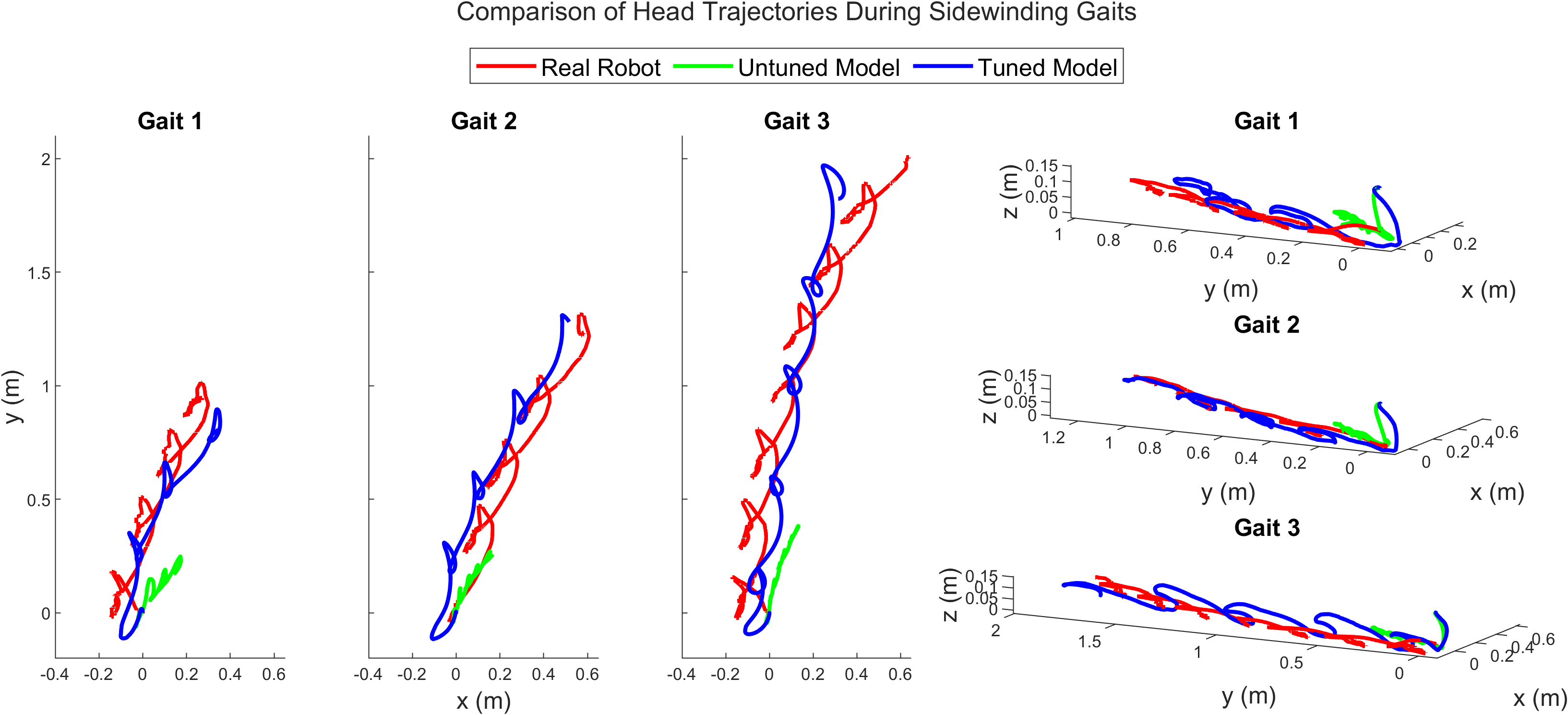
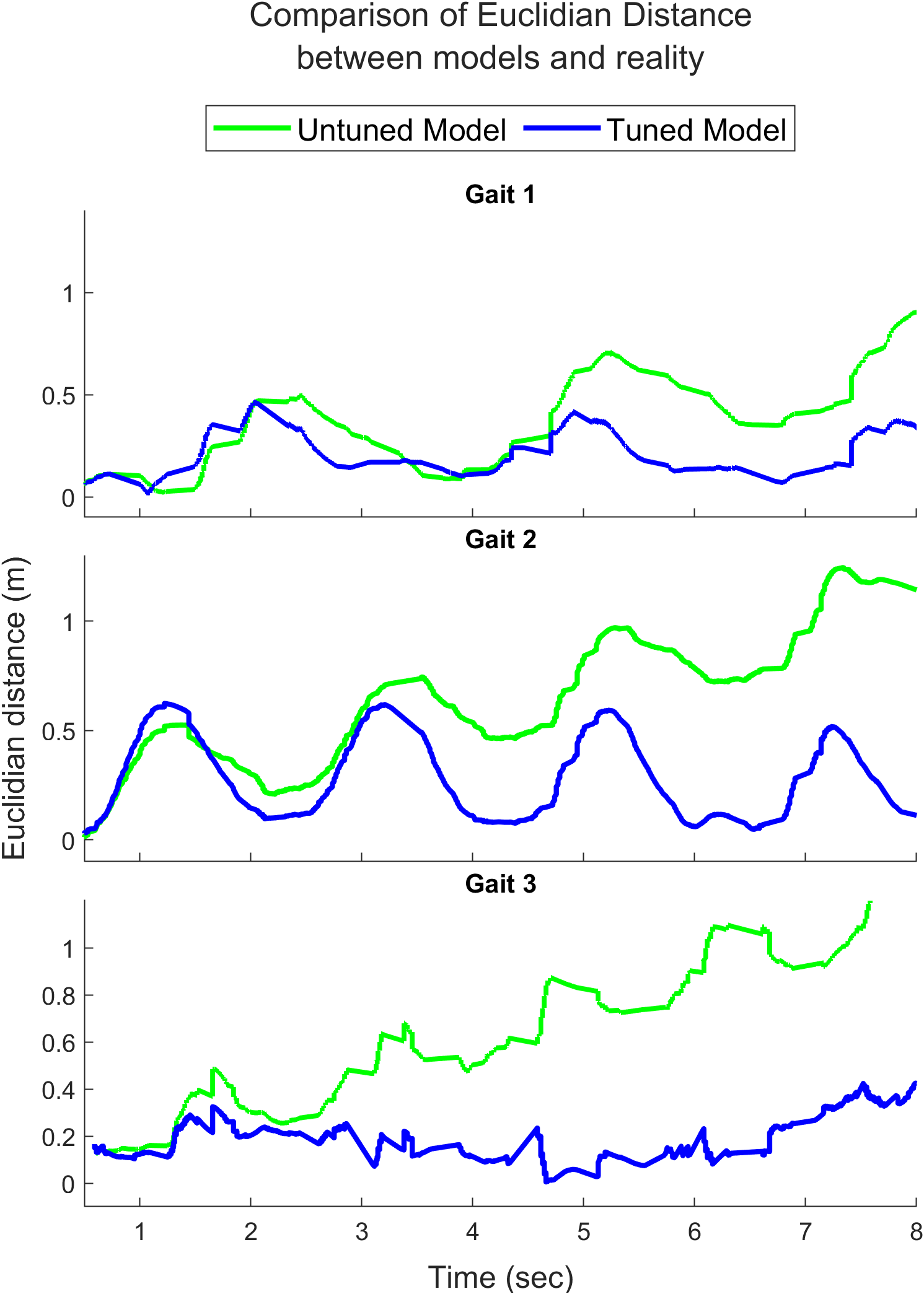
Figure 13 shows the alignment in the trajectories of the robot’s middle and tail links while performing the three gaits. Figure 15 (left) provides a quantitative comparison between the tuned and untuned models using the Euclidean distance metric, measuring the distance between the real and simulated robot’s head positions during gait execution. The error reduction is significant after tuning, especially for gaits 2 and 3. For gait 1, at a lower frequency of 0.35 Hz, the untuned model performs comparably to the tuned model due to minimal movement.
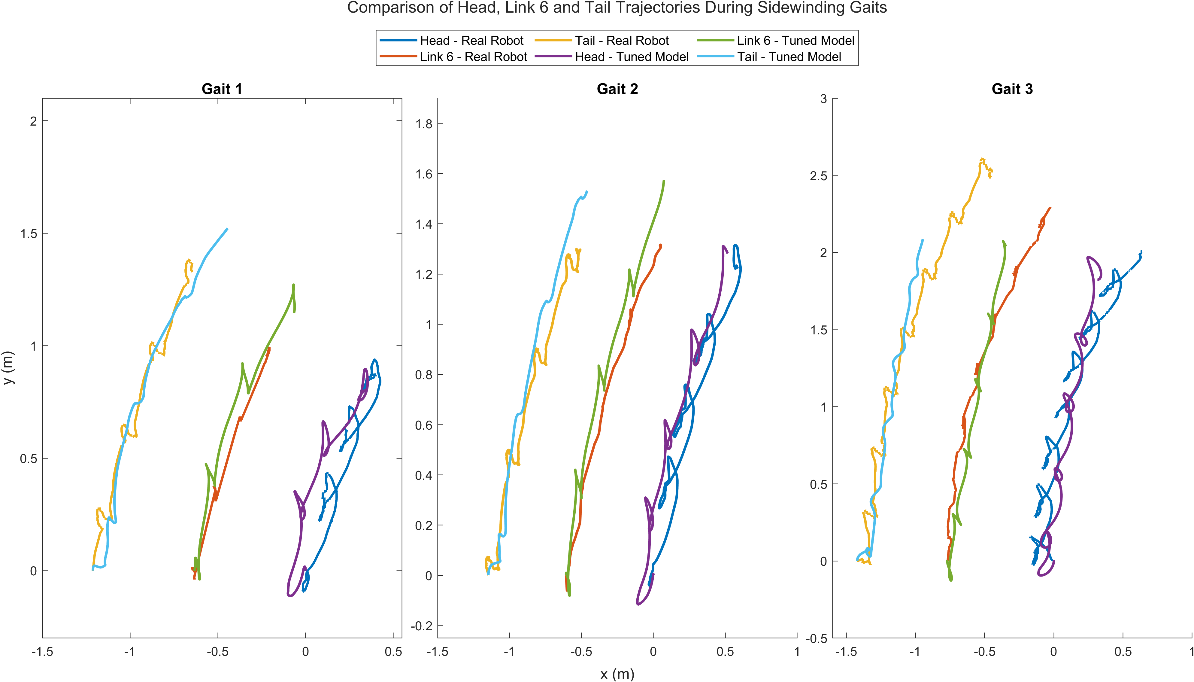
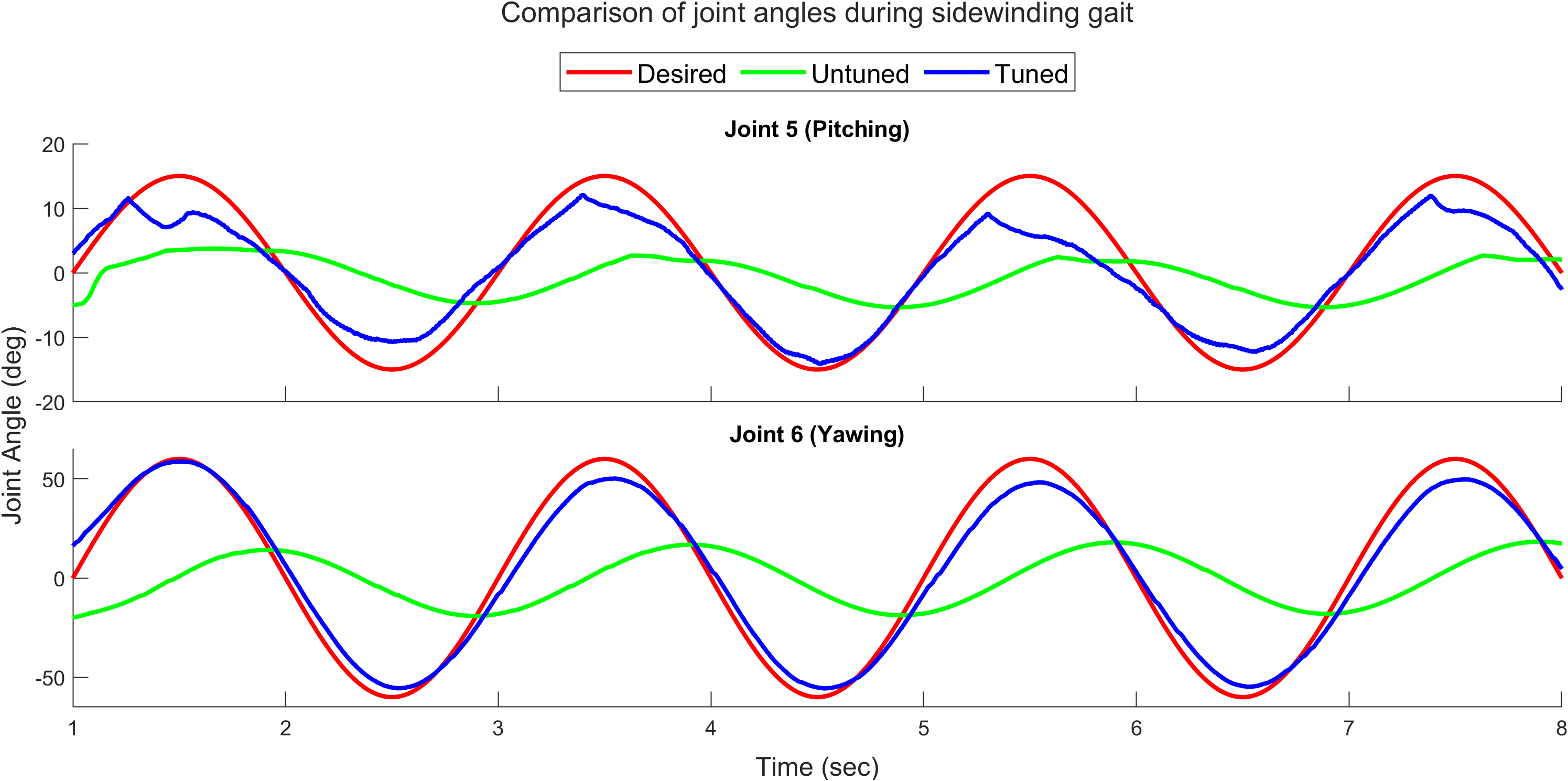
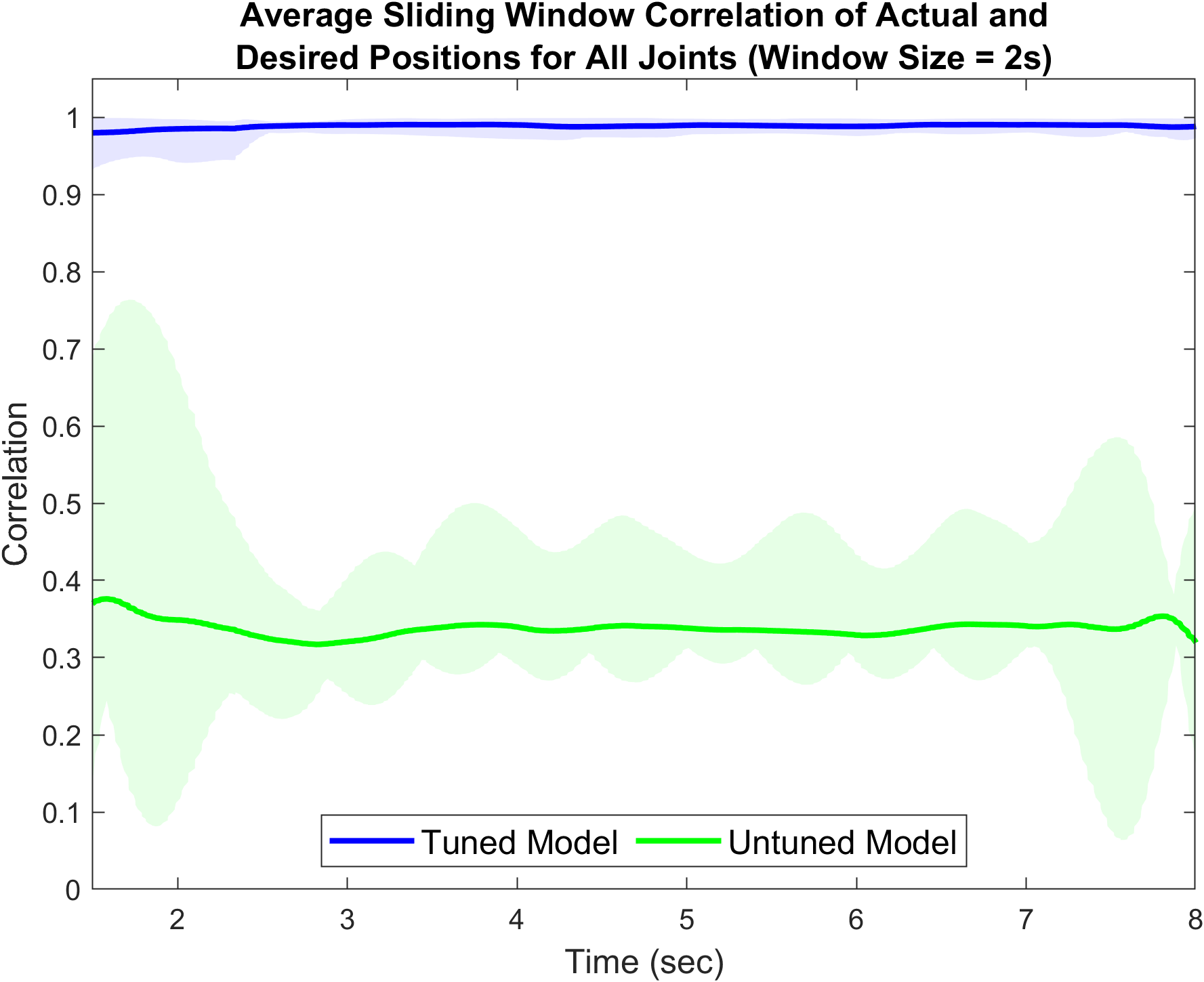
Figure 14 compares joint angles for joints 5 and 6 during a sidewinding gait at 0.5 Hz, showing improved agreement between the real robot and the simulator after tuning. Figure 15 (right) further supports this with a comparison of the average sliding window correlation across all 11 joints. The tuned model achieves a correlation factor close to 1.0, indicating strong alignment, while the untuned model’s correlation factor is around 0.35, indicating a significant performance gap.
Loco-manipulation Controller
Video 5 illustrates the successful execution of our algorithm for locomanipulation in the Webots simulator. The robot and object start at random positions, and the algorithm moves the object to a set goal. Video 6 and 7 show the algorithm handling different configurations of robot, object, and goal positions. When the object deviates from its path, the robot adjusts by turning while moving the object, ensuring it reaches the goal directly.
Video 8 demonstrates the algorithm’s ability to perform loco-manipulation in a dynamic environment. Initially, the algorithm directs the object toward the goal, but when the object’s position changes, the algorithm adjusts its path and successfully guides the object to the new goal position.
An episode is deemed successful if the robot moves the object to the goal within 700 steps. After 200 episodes, the average success rate and the average number of steps taken were calculated and are shown in Table 2.

Conclusion
My work significantly advances the sim-to-real problem on the COBRA platform by developing a robust model matching framework. This framework effectively aligns the behavior of the COBRA robot in the Webots simulator with its real-world performance across various gaits, achieving substantial improvements in simulation accuracy with minimal tuning. The framework’s scalability allows for additional simulator parameters to be fine-tuned as needed, and its modular design enables application to different robotic morphologies, such as quadrupeds and bipeds. This reduces the need for extensive real-world testing, minimizing wear and tear on physical robots and cutting costs. Comprehensive evaluation metrics further ensure a thorough assessment of the tuned model’s performance across different scenarios and gait types, enhancing the reliability and efficiency of robot simulation.
The loco-manipulation algorithm, with a high success rate of 94.3%, demonstrates robustness and reliability in diverse environments. Its versatility makes it valuable for applications such as disaster response, where it can clear debris, and space exploration, where precise object manipulation is crucial. This algorithm enhances COBRA’s capabilities in disaster response, space missions, and industrial automation, addressing complex challenges and advancing robotic systems in real-world scenarios. By leveraging this algorithm, COBRA can significantly improve efficiency, completing tasks with minimal errors.